Long Short-Term Memory Network

To determine if deep learning performs better than machine learning in the traffic classification task, in community networks, three key research questions need to be answered:

• Which of the deep learning architectures provides the highest classification accuracy subject to the resource constraints found in a community network?
• Does the more complex Long Short-Term Memory (LSTM) network sufficiently outperform the simpler Multi-Layer Perceptron (MLP), assuming the same computational constraints?
• Does the best deep learning network sufficiently outperform a traditional machine learning model, the Support Vector Machine (SVM), assuming the resource constraints found in a community network?

The success of the project will be determined by how well these research questions were answered.

To answer the research questions two experiments were set up to test the different model's accuracy and speed over a range of possible time and memory constraints. This section describes those experiments.

Accuracy

The deep learning models' performance will need to be compared subject to memory constraints. The number of parameters in a model is directly proportional to the amount of memory needed by the model. Therefore, this was used as the metric to compare memory efficiency. For each of the deep learning model architectures, MLP and LSTM, the number of parameters in the architecture will be varied and the test accuracy will be calculated. The number of parameters in each architecture will range from 15 000 to 1 000 000. This will allow the models to be compared at high and low memory constraints. So if a community network can only have a model with 100 000 parameters it will be easy to see which architecture will perform the best. The SVM has a constant number of parameters so the accuracy for the SVM will be reported for the best performing SVM model.

Speed

For each model architecture, and at each of the different parameter levels, the average time it takes to make a prediction and the number of packets classified per second will be calculated. This will allow time constraints to be placed on the models, which will make it easy to see which type has the best accuracy under those time constraints. It will also determine whether the deep learning models can support real time classification. Since the SVM has a constant number of parameters, the number of packets classified per second will be calculated for the best performing SVM.

Accuracy

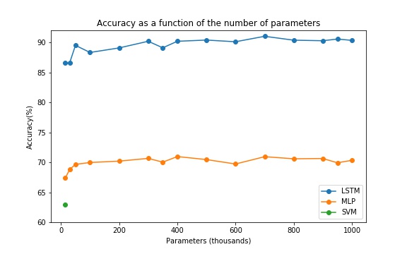
The first research question was to determine whether the LSTM could attain a higher accuracy when compared with the MLP. The second research question was to check that the increase in accuracy was significant enough to warrant using the added complexity. In the plot the points represent the test accuracy calculated for a given parameter level. The figure makes it clear that the LSTM outperforms the MLP in predictive power across all parameter levels. The LSTM’s accuracy ranges form 86.5% to 91% and the MLP’s accuracy ranges from 66.8% to 70.5%. There is some noise in the accuracy because the optimization process for neural networks is stochastic but the difference between these two models is large enough to say that the LSTM performs sufficiently better under every memory constraint. This was expected because the LSTM is far more suited to learning sequential information, and the byte stream of a packet is inherently sequential. It is also good to note that there does seem to be a general relationship between the number of parameters and the accuracy. With the accuracy increasing at a decreasing rate as the number of parameters increase. The third research question was trying to determine whether the best deep learning model sufficiently outperforms a traditional machine learning model, the SVM. Since the SVM has a constant number of parameters the test accuracy was given for the best performing SVM model. This accuracy is represented on the plot by the green dot. It is clear that the LSTM performs far better than the SVM across all memory constraints.

Speed

This section will present the results of the speed tests. These results will help us determine which of the deep learning models has the fastest prediction speed, and whether these models can be used for real time classification. The figure shows the results from the speed tests done for the MLP and the LSTM. The results are presented as the number of packets that can be classified in a second. It can be seen that there is some noise in the data, this comes from the stochastic nature of timing how long it takes to run a section of code. For each parameter level, the LSTM’s times were averaged over 7000 samples and the MLP’stimes were averaged over 10 000 samples, to reduce the noise as much as possible. Even though there is noise in the data, it is clear that the MLP can classify more packets a second than the LSTM. The number of packets the MLP can classify per second ranges from 25.5 to 26.6 and for the LSTM the range is 19.7 to 24.3. Due to the sequential structure of LSTM network, it is not surprising that it runs more slowly than the MLP, which can be parallelised more easily. The plot also shows that as the number of parameters increase, there is a decrease in the number of packets classified per second. However, what is quite interesting is that the MLP’s decrease is linear while the LSTM decreases at a much quicker rate. This is probably due to the increase in the number of calculations done per sequential step in the LSTM. It must also be noted that the smallest number of packets classified per second was 19.7 which is fast enough for real time classification. The SVM was able to classify approximately 3846 packets per second.

Batch Test

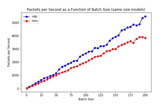
The time it takes a model to make a prediction was calculated for only a single packet, but waiting and classifying multiple packets at the same time can reduce the time it takes to make a single prediction. This is called batch predicting. The plot shows the relationship between the batch size and the predictions made per second. The dots in the plots represent the the average number of packets classified per second, for a given batch size. The MLP and LSTM used in the plot both had 700 000 parameters. These plots clearly show that increasing the batch size allows for faster predictions. This is because the prediction function gets run in parallel, which reduces the overhead found when predicting only a single packet. This plot also shows that the LSTM is slower than the MLP, accross all batch sizes. Batch predicting can help increase the prediction speeds of the deep learning models without having to change the architectures and compromise the accuracy.

Since this project focuses on real time classification it was important to determine if the deep learning architectures could perform real time classification. The speed tests showed that even the slowest deep learning models were able to classify enough packets per second to be consisdered for the real time classification task. If network managers need faster prediction speeds but do not want to compromise the accuracy by making the models smaller, they could use batch predictions. The batch tests show that bacth predictions can offer a large speed-up, by taking advantage of parallelization of the predict function. They also show that the prediction speeds increase for increasing batch sizes, which could prove vital if there is a large amount of traffic coming in at the same time.

The LSTM architecture attained the highest classification accuracy of 91%, and significantly outperformed the MLP across all memory constraints. These results answered research questions one and two because it showed that the LSTM is the best deep learning architecture, and it showed that it sufficiently outperformed the MLP when resource constraints were applied. The MLP and the LSTM were also able to obtain a sufficiently higher classification accuracy than the SVM, even under the most strict memory constraints. This answered the final research question because the best deep learning architecture outperformed the SVM even when it was subject to resource constraints. The high accuracy obtained by the LSTM gives evidence that the data found in packets is sequential, and architectures that are built to process this information will do better in the packet classification task.