One-Dimensional Convolutional Neural Networks
Overview
Networks that support Quality of Service (QoS) configuration require an online network traffic classification tool to separate individual packets into their respective application classes at the network gateway. Machine learning techniques have proven to be effective for this classification task, even when the traffic is encrypted or routed through a VPN. Out of the machine learning techniques considered, deep learning models have typically attained the highest accuracy in research on traffic classification. However, research has not extensively considered the performance requirements of the models trained, incentivizing the development of larger, slower models in pursuit of higher accuracy. This poses a problem for online classification, particularly in low resource environments, where classification must be near instantaneous to avoid introducing unnecessary latency. This paper considers the trade-off between prediction speed and accuracy for the packet-based network traffic classification task by developing a framework that builds and compares hundreds of 1D CNN and MLP deep learning models of various sizes with varying payload lengths used as input. These deep learning models are further compared to an SVM across the same metrics. The models are evaluated using six different sets of hardware constraints that might be found in a modern community network, and the model that achieves the highest accuracy is selected for each of these resource environments, subject to it classifying the traffic efficiently enough. The study finds a clear trade-off between prediction rate and attainable accuracy. In this regard, it is only for resource environments with an exceptionally slow CPU that an SVM should be used. For low to middle-range CPUs an MLP can be used, and for the most powerful of CPUs, a 1D CNN is the preferred model.
Experiment Procedure
Varying the input length
A method is written to transform the input data to the input lengths under consideration so that the models can be built and evaluated on inputs of varying sizes.
Establishing a baseline with SVM
The first step of the experiment involves setting a baseline classification accuracy on the dataset with a traditional machine learning model using the scikit learn LinearSVC library (SVM classifier). The model was trained and evaluated across all 4 input lengths specified. A linear kernel along with a one-vs-the-rest scheme is used as per the scikit-learn documentation.
Training deep learning models
300 MLP and 1D CNN models are trained across the hyperparamater and model architecture search space for each of the 4 input lengths outlined in section 4.4 using Keras with Tensorflow. This results in 1200 different MLP models and 1200 different CNN models that can be evaluated. The hyperparameters chosen for each of these models are saved to a csv file and the model itself is also saved. Early stopping is used to reduce training time and provide a regularization effect. A Tela V100 GPU is used to do this training and it takes between 24 and 48 hours to train each set of 1200 models.
Performance evaluation
The models are now loaded into a CPU instance where their prediction speed on the test set of 20 000 packets is recorded using a batch size of 32. The prediction speed is added to the csv file generated above, along with the size of the saved model in megabytes. The hardware specs for the CPU instance used is retrieved with a bash script and saved to a text file for later consideration.
Comparison to hardware constraints
A python script is written to take a csv file containing the model prediction speeds and the effective processing power of the system that produced that prediction speed. The ratio between the clock speed on the system that the model was tested on and the hardware constraints under consideration is calculated and the prediction rate is scaled by that same ratio. Thereafter, the calculated prediction rate is reduced by 75% to account for the assumption that only 25% of the system's resources should be allocated to the traffic classification. The prediction rate is now compared to the required throughput to see if the hardware under consideration can support the model. An example showing how this is calculated is included in the appendix for additional clarity.
Results
SVM Accuracy and Prediction Rate
The SVM is capable of predicting at an accuracy of just under 65% when the full payload is used as the input. The prediction rate improves as the number of bytes included decreases, showing the improvement in performance of considering less features. However, this comes at the cost of a decrease in accuracy of just over 15% as soon as the full payload of 1460 bytes is no longer considered. There does not seem to be a significant difference between the accuracy of the SVM models that use less than the full payload, suggesting that the model does not extract any additional useful information from bytes 365 to 1095.Model Accuracy Comparison
The figure shows the difference between the distribution of accuracy on the test set for each of the deep learning models using each of the input lengths considered. It is clear that models with the full payload are capable of achieving a higher accuracy than models that use less bytes as input, but there does not seem to be a significant difference between the accuracy attainable for input lengths of any other size. The higher accuracy achieved by the 1460-byte models could be attributed to either some very useful features in the later bytes in the payload or that the payload length is a useful feature that the models can only learn when they have the full payload.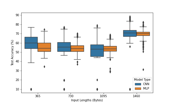
Model Prediction Rate Comparison
The figure provides insight into the differences between the prediction rates of the MLP and the 1D CNN, as well as the differences between the prediction rates of models trained with the different input lengths. It is clear from the diagram that the CNN is considerably slower than the MLP across input lengths of all sizes. Additionally, a trend of models performing faster with a smaller input length can be seen for both the MLP and CNN.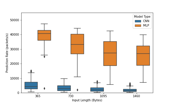
Maximum Accuracy Attainable by Input Length
The figure shows the maximum accuracy that each model class can attain for each input length. The highest accuracy attained by every model class was done with the full payload, indicating that the full payload should be used if accuracy is the only concern. However, section 5.3 showed that considering less features can result in a faster prediction rate, so it is possible that using a smaller payload could be beneficial for some hardware-model combinations. There does not seem to be a significant difference between the highest accuracy attainable for models with between 365 and 1095 bytes as input, suggesting that bytes 365 to 1095 do not add significant information.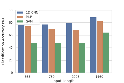
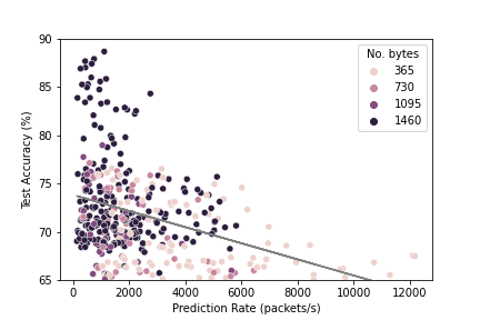
Relationship Between Accuracy and Prediction Rate
The figure below shows the relationship between the test accuracy attainable and the prediction rate for the MLP models. There appears to be an inverse relationship, with the models attaining a higher accuracy at the cost of a slower prediction rate. The number of bytes considered by each model is also shown by adjusting the hue of the dots. A trend of the dots getting darker as the accuracy improves and then prediction rate declines can also be observed, indicating that the smaller input sizes demonstrate faster classification at the expense of accuracy for the MLP models.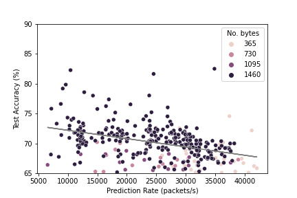
Model Allocations by Hardware Constraints
The table shows which model was chosen for each hardware system, where the model with the highest classification accuracy is chosen subject to it meeting the required prediction speed on the given hardware system. Firstly, it is only the weakest processor that resorts to using an SVM with an accuracy of 64.59% and only the most powerful processor that selects a CNN with an accuracy of 84.29%. The others all use the same MLP model with an accuracy of 82.48%, aside from the second weakest processor which uses an MLP with 365 bytes as input and produces an accuracy of 72.16%. The highest accuracy CNN is too slow even for the fastest CPU considered.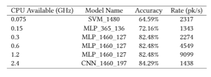
Conclusions
Highest Accuracy Model Performances
Similar to related literature, the 1D CNN has performed better than the MLP on accuracy. However, it is significantly slower than the MLP, with the highest accuracy 1D CNN predicting 30 times slower than the highest accuracy MLP. The highest accuracy 1D CNN achieved an accuracy of 88.64% and the highest accuracy MLP achieved an accuracy of 82.48%. The best SVM model uses the full payload as features and achieves an accuracy of 64.59%, significantly worse than the CNN and MLP, but performs 6 times faster than the best MLP and 180 times faster than the best 1D CNN. The highest accuracy 1D CNN is too slow for even the fastest of the resource constraints considered.
Inverse Relationship between Prediction Rate and Test Accuracy
It has been shown that there is a general inverse relationship between the prediction rate and the attainable accuracy, both within model classes and between model classes. This means that low-resource environments may have to select a faster model with a lower accuracy to meet the throughput requirements of an online traffic classifier.
Full Payloads Achieve Higher Accuracy at the Cost of Performance
The analysis on considering payload lengths of less than the full 1460 bytes revealed that this does come at a significant accuracy cost, but with a faster prediction rate. Despite performing worse than full-payload models, the models with 365, 730, and 1095 bytes as features performed similarly to each other, suggesting that there is not meaningful information captured from bytes 365 to 1095. Despite the lower accuracy, considering smaller input lengths can be worthwhile lower resource environments as is shown by MLP_365_136 which only uses the first 365 bytes as input and was selected for the second slowest resource environment.
Community Network Recommendation
The recommended model for a given community network depends on their required throughput, available processor resources, and available RAM. Only the first two have been considered here, but it is reasonable to infer that models with a faster prediction rate will generally require less RAM as less calculations are performed and thus less values need to be stored. For most community networks, it appears that the MLP is a good option for network classification as it seems to perform sufficiently fast to meet the processor constraints of most community networks while achieving a reasonable accuracy. The SVM should only be used in community networks that have exceptionally slow processors. The CNN should be used in community networks with high-end CPUs or access to a GPU. The process of selecting a model can be easily replicated for a network with arbitrary resource constraints as a function has been written that will take the constraints specified and return the model that can attain the highest accuracy subject to the constraints. For actual implementation in a community network with known resource constraints, this paper can serve as a guide as to what sort of models could be supported by the network and a model could be fine-tuned to achieve an accuracy marginally higher than the ones generated by the random search in this paper.