Overview
Data Pre-Processing
We obtained time series data of the daily prices of three various financial equities.
We obtained this data from finance.yahoo.com.
 https://www.forex.academy
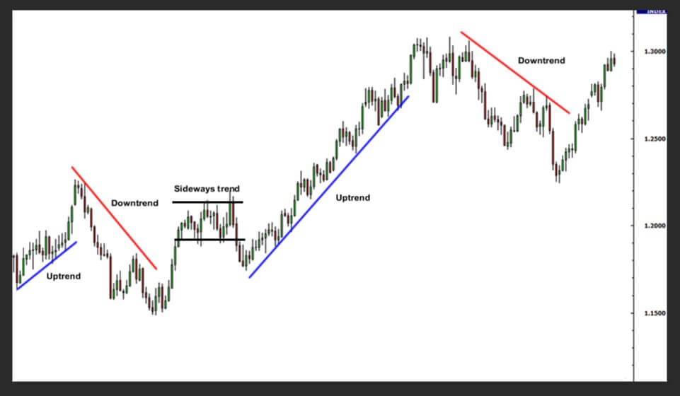
Similar to the image above,
we systematically converted this raw time series data into a sequence of trend lines for each financial equity.
Since we are concerned with teaching a machine learning model to predict the next trend it is clear that we are dealing with a supervised learning problem.
Thus we needed to construct our data (the sequence of trend lines) into a collection of input-output pairs, otherwise known as feature-label pairs.
To this end we used a standard sliding window algorithm. In order to construct a single input-output pair the algorithm groups trend lines into a matrix of four trend lines and associates a label where the label is the next trend line.
The algorithm does this for the entire data-set as depicted in the picture below.
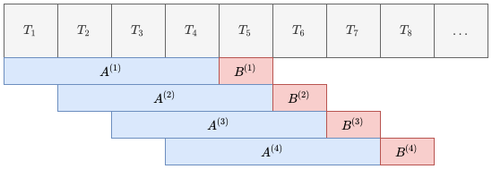 This algorithm groups trend lines (T) into a matrix of four trend lines (A) and associates a label (B) where the label is the next trend line.
Machine Learning
 http://brainstormingbox.org
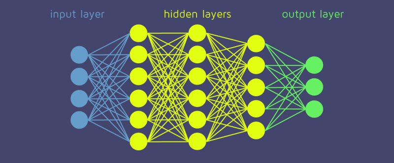
As described above, we are dealing with a supervised learning problem. In order to train the weights of the machine learning model we use 60% of the trend lines constructed (explained above).
We then pass the four previous trend lines into a machine learning model and the output of the machine learning model is the predicted next trend line.
Automated Machine Learning
We applied a subset of Automated Machine Learning to this task known as Combined Algorithm and Hyper-Parameter Selection (CASH).
That is, for a pre-defined selection of machine learning algorithms and a selected range of their respective hyper-parameters - we try to find the combination of algorithm and hyper-parameters that best predicts the next trend line.
This CASH problem can be seen as a black-box optimization problem, i.e. there is a large search space, we are trying to find the location in this search space which minimises the objective function.
In our case the objective function used is the combined (Trend Line Length and Trend Line Gradient) mean squared error of actual observed trend lines versus predicted trend lines over a validation set (The validation set used is a subset of 20% of the trend lines constructed above).
Evolutionary Optimization Algorithms
Now that we have set up a large search space and an objective function over that search space - we are left with a difficult optimization problem!
 Pablormier - https://pablormier.github.io/2017/09/05/a-tutorial-on-differential-evolution-with-python
A class of optimization techniques known as Evolutionary Optimization Algorithms are a promising candidate to perform very well for this task.
The main concept of an Evolutionary Optimization Algorithm is generations. A generation contains a population of members where each member represents a position in the search space.
Through variations of mutation and selection techniques - a new generation is born - where the new generation is supposedly an improved version compared to its parent generation.
In this way the algorithm attempts to find the best position.
The focus of our research is the exploration of two Evolutionary Algorithms in particular, namely: Genetic Algorithms and Differential Evolution.
Goals

The focus of this research was framed in a single research objective which we set out to acheive. Our objective was to analyse and compare the performance of evolutionary algorithms for hyperparameters optimisation in neural network models given the context of trend prediction in time series data.
Thus, we set out our research to answer two research questions formulated from the above objective. Firstly, can evolutionary algorithms be used to effectively solve the hyperparameter optimisation problem when compared to a conventional method - random search in this case - in terms of minimising the validation mean squared error of the model? Secondly, how well do the models produced by the evolutionary algorithm AutoML method perform in the task of trend prediction, using the model's test mean square error as the evaluation metric?
Genetic Algorithm Objectives
The experiments regarding genetic algorithms were evaluated further with the objective of understanding how well the two algorithms (genetic algorithm and random search) perform under both high and low computational budgets.
Differential Evolution Objectives
The experiments regarding Differential Evolution had two primary objectives.
The first objective was to study the effect of change in the control-parameters of the Differential Evolution algorithm in order to optimize its performance.
The second objective was to compare the performance (in terms of speed of minimisation and ability to learn the underlying pattern of the data) of differential evolution to an unintelligent random search and to another state of the art evolutionary algorithm.
Results
In order to acheive the objectives outlined at the beginning of our research, we performed a number of different experiments. We implemented the experiments using Python along with PyTorch for the neural networks and PyMoo for the evolutionary algorithm. We evaluated the evolutionary algorithms against a hand-made random search method. Below are the details and the results pertaining to each evolutionary algorithm under evaluation.
Genetic Algorithm
In order to evaluate the performance of the genetic algorithm against the random search algorithm, two sets of experiments were performed. We performed experiments with both high and low computational budgets in order to evaluate the AutoML algorithms under different computational circumstances. These experiments were performed on two datasets - the closing prices of the NYSE and NASDAQ. Each of these experiments were run 8 times in order to have robust results. We evaluate the performance of the genetic algorithm and random search by means of the validation MSE on two different neural network models - an LSTM and an MLP.
Results
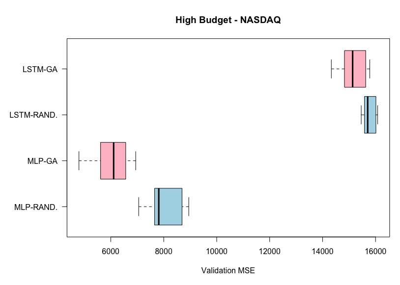 Results from high budget experiments on the NASDAQ dataset. Lower MSE is better.
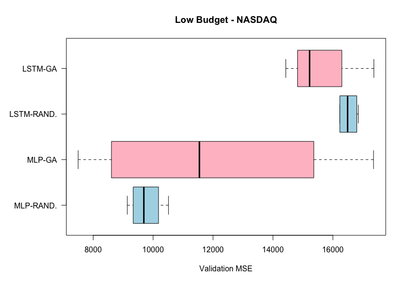 Results from low budget experiments on the NASDAQ dataset. Lower MSE is better.
From the first plot, we can see that the genetic algorithm outperforms the random search algorithm, on average, for both the MLP and the LSTM in the high budget experiments on the NASDAQ dataset. This is not the case for the low budgets experiments where random search outperforms genetic algorithm on the LSTM. It is also important to note the lower variability of the genetic algorithm experiments on the high budget experiments, but the opposite case in the low budget experiments.
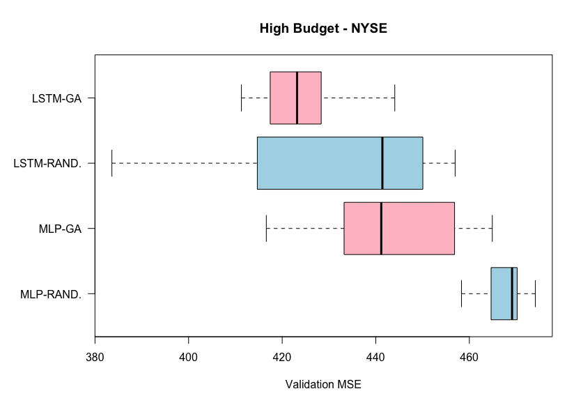 Results from high budget experiments on the NYSE dataset. Lower MSE is better.
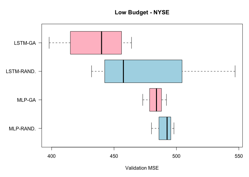 Results from low budget experiments on the NYSE dataset. Lower MSE is better.
From the above two plots for the experiments on the NYSE dataset, we can see that the genetic algorithm outperforms the random search algorithm, on average, for both the MLP and the LSTM. This is the case for both the high and low budget experiments. However, here the variability is varied betweem the two AutoML methods.
Conclusions
From the results of the experiments, we found that a genetic algorithm can, in general, outperform a simple random search algorithm for the task of hyperparameter optimisation given both high and low computational budgets. However, the time to terminate for the genetic algorithm was significantly longer than random search.
The performance of the models selected by the AutoML algorithms were poor on out-of-sample data. This was determined to be due to the nature of our validation process, rather than the autoML techniques themselves.
Differential Evolution
In line with Objective one concerning Differential Evolution - we found that a population size of 20 performed very well.
By opting to choose a lower a population size we were able to still have many generations within our budget.
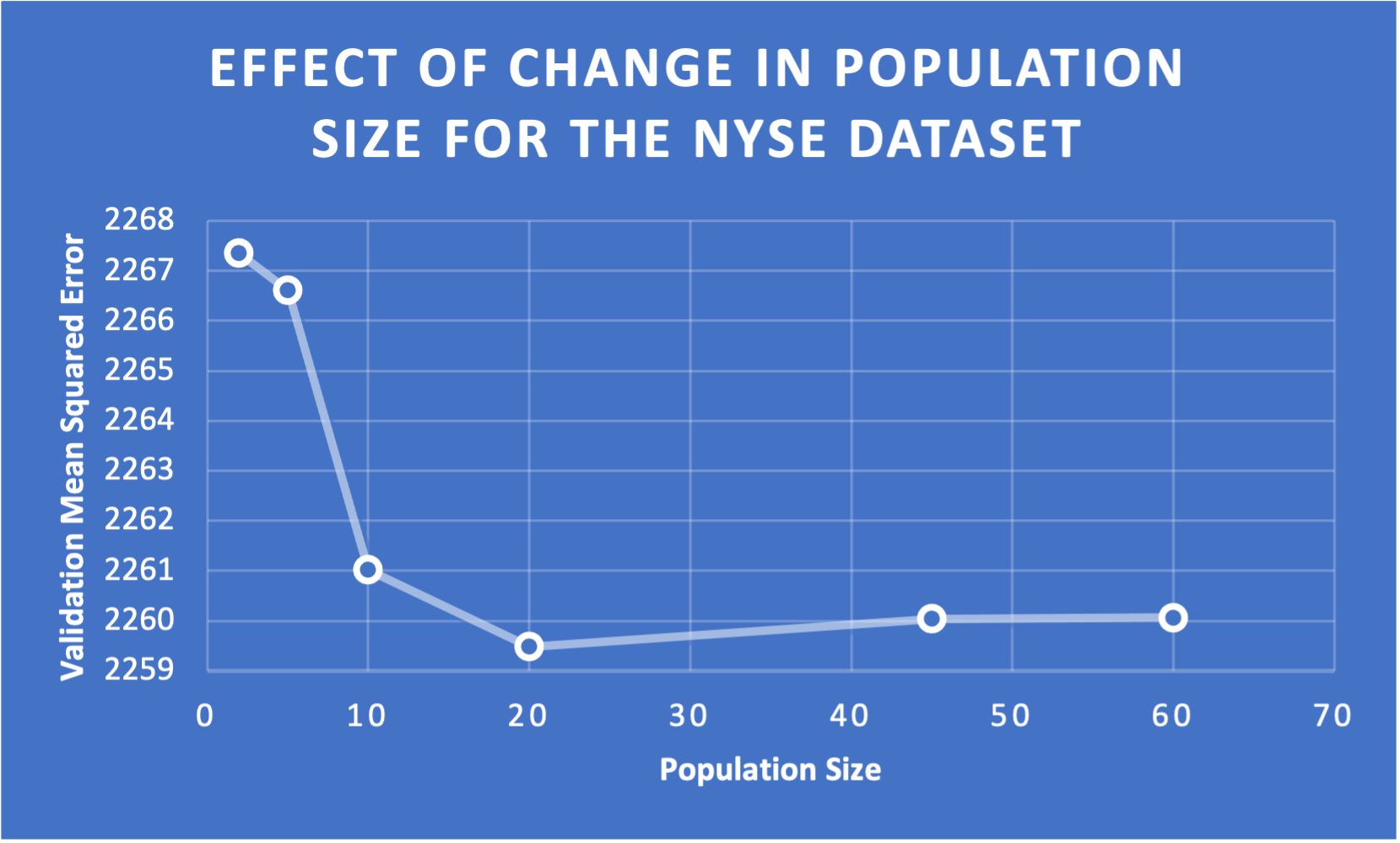 This image clearly depicts the drop in mean squared error with a validation size of 20.
However, as shown in the picture below, no obvious improvement could be found by tweaking the F and CR control-parameters.
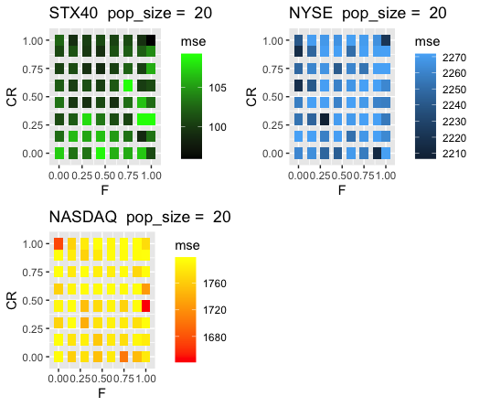 This image clearly depicts the drop in mean squared error with a validation size of 20.
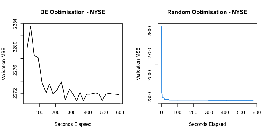
After selecting optimal control-parameters, Differential Evolution was evaluated in how quickly it was able to minimize the objective in comparison to a random search and a different state-of-the-art evolutionary algorithm.
As can be seen in the image below, Differential Evolution showed to be more effective than a completely random search in efficiently minimizing the objective function.
This image clearly depicts the drop in mean squared error with a validation size of 20.
After selecting optimal control-parameters, Differential Evolution was evaluated in how quickly it was able to minimize the objective in comparison to a random search and a different state-of-the-art evolutionary algorithm.
As can be seen in the image below, Differential Evolution showed to be more effective than a completely random search in efficiently minimizing the objective function.
 However, when the final models were evaluated on a set of out-of-sample data, the model found by the Differential Evolution algorithm was not superior to that found by Pattern Search or even the unintelligent random search for any of the data sets.
Docs
Contact
James Taljard
Department of Computer Science
University Of Cape Town
Elements
Text
This is bold and this is strong. This is italic and this is emphasized.
This is superscript text and this is subscript text.
This is underlined and this is code: for (;;) { ... }. Finally, this
is a link.
Heading Level 2
Heading Level 3
Heading Level 4
Heading Level 5
Heading Level 6
Blockquote
Fringilla nisl. Donec accumsan interdum nisi, quis tincidunt felis sagittis eget tempus
euismod. Vestibulum ante ipsum primis in faucibus vestibulum. Blandit adipiscing eu felis iaculis
volutpat ac adipiscing accumsan faucibus. Vestibulum ante ipsum primis in faucibus lorem ipsum dolor
sit amet nullam adipiscing eu felis.
Preformatted
i = 0;

while (!deck.isInOrder()) {
    print 'Iteration ' + i;
    deck.shuffle();
    i++;
}

print 'It took ' + i + ' iterations to sort the deck.';
Lists
Unordered
- Dolor pulvinar etiam.
- Sagittis adipiscing.
- Felis enim feugiat.
Alternate
- Dolor pulvinar etiam.
- Sagittis adipiscing.
- Felis enim feugiat.
Ordered
- Dolor pulvinar etiam.
- Etiam vel felis viverra.
- Felis enim feugiat.
- Dolor pulvinar etiam.
- Etiam vel felis lorem.
- Felis enim et feugiat.
Icons
Actions
Table
Default
| Name |
Description |
Price |
| Item One |
Ante turpis integer aliquet porttitor. |
29.99 |
| Item Two |
Vis ac commodo adipiscing arcu aliquet. |
19.99 |
| Item Three |
Morbi faucibus arcu accumsan lorem. |
29.99 |
| Item Four |
Vitae integer tempus condimentum. |
19.99 |
| Item Five |
Ante turpis integer aliquet porttitor. |
29.99 |
|
100.00 |
Alternate
| Name |
Description |
Price |
| Item One |
Ante turpis integer aliquet porttitor. |
29.99 |
| Item Two |
Vis ac commodo adipiscing arcu aliquet. |
19.99 |
| Item Three |
Morbi faucibus arcu accumsan lorem. |
29.99 |
| Item Four |
Vitae integer tempus condimentum. |
19.99 |
| Item Five |
Ante turpis integer aliquet porttitor. |
29.99 |
|
100.00 |