Data Preprocessing
Obtaining SANREN Data
The first step in conducting our research was to obtain times- series network traffic data from SANREN. This data was accessed through the University of Cape Town. The data is stored as tab-separated .csv files, and each data set consists of a multitude of variables, each describing the quality of the network traffic flows on SANREN over a measured period of time. The SANREN data has been placed on a data store at the University of Cape Town - which is available to be accessed remotely. However, for this research project, a smaller 47000- observation sample was used to train, validate and test the LSTMs that this paper evaluates. An example of the format of the SANREN data is provided on the right. The response variable for this project is Bytes per flow.
Data Engineering
The raw SANREN data has to be extracted and cleaned for a neural network model. This preprocessing step transforms. raw data into input for each of the neural network models. Initially, the categorical features were encoded using one-hot encoding - which creates a new binary column for each instance of a categorical variable - however, this caused the DataFrame’s dimensions to increase dramatically and had little impact on the predictive power of the LSTM models - so the categorical variables were subsequently dropped from the DataFrame.
Additionally, to capture the relationship between South African university schedules and network traffic data, two new variables were engineered. The first is a Simple day variable - which numerically encodes the day of the week - and the second is a binary holiday variable - which asserts whether the network flow occurred during a university holiday or not. The holiday dates were defined by the University of Cape Town’s academic schedule for 2020. Byte values were encoded to 64-bit float representations, strings were removed - as strings are not acceptable input for a TensorFlow LSTM - and temporal values were encoded to 64-bit integer nanosecond representations.
| Variable | Example Value |
|---|---|
| Date | 2020-07-04 |
| First-seen | 20:10:06.480 |
| Duration | 1.223 |
| SrcIP | 146.231.4.0 |
| DstIP | 155.232.240.0 |
| Packets | 4500 |
| Bytes | 234000 |
| pps | 3679 |
| bbs | 1.5 M |
| Bpp | 52 |
Preliminary Data Analysis
To provide insight into the underlying patterns, correlations and composition of the SANREN data, a preliminary statistical analysis was performed.
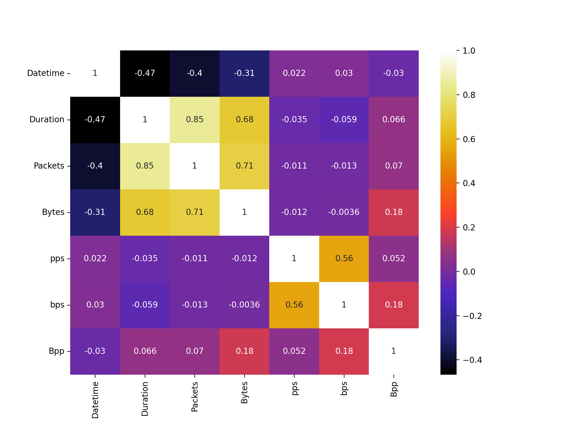
To investigate the possibility of multicollinearity, a correlation matrix was plotted. There are strong correlations between Bytes, Packets and Duration. The option of removing all of the variables apart from the three that make up the stronger, yellow correlations in the upper left of the matrix was considered, although due to the non-linearity of the data, this design decision was rejected. Other correlative relationships of interest are the negative relationship between Bytes and Datetime and the strong positive relationship between Duration and the response. In this sample, the weak correlation between Bytes and Datetime suggest that the byte volume per flow is decreasing as time increases. Importantly, this does not imply that there is less network traffic in general because network traffic volume is a function of byte per flow as well as the number of flows. The relationship between Bytes and Duration implies that longer flows generally have more data being transferred - which is a sensible assumption.
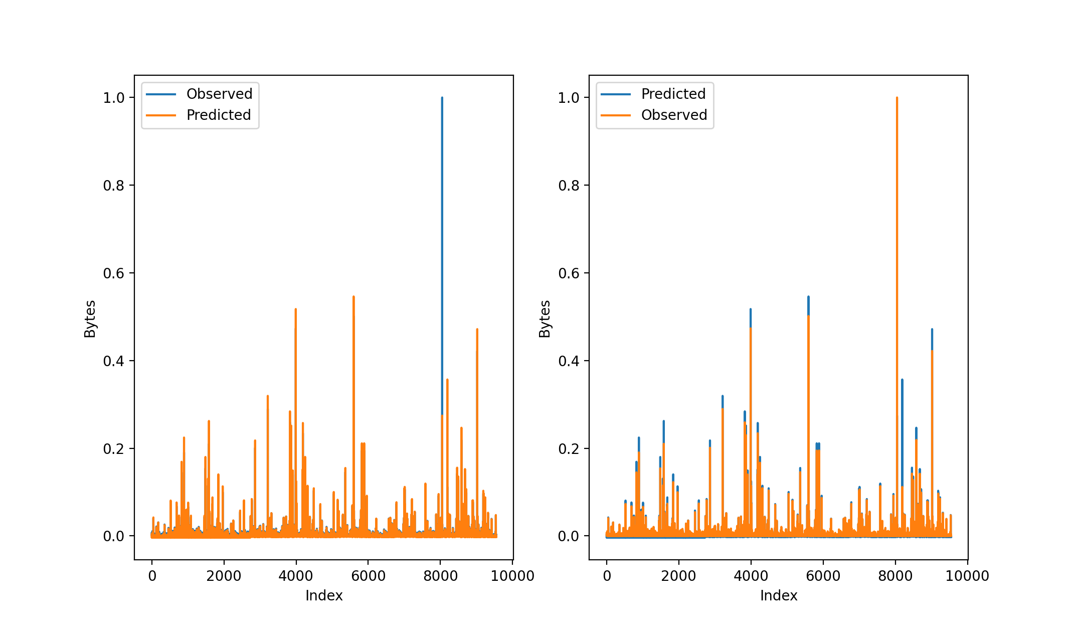
The preliminary data analysis provides an opportunity to garner insight into whether SANREN traffic data varies with time and day in relation to the South African university calendar. To extract the relationship between time of day, university holidays and byte volumes, a pair of scatter plots were fitted. The figure on the left show the total byte flows over each day of the week. Surprisingly, there is noclear distinction between bytes flows during the week compared to the weekend. Similarly, the total byte flow per per type of day is shown. Again, it is surprising to see that the total byte flows are higher on average during a holiday. This is unexpected, as the SANREN links research units and other university-related institutions.
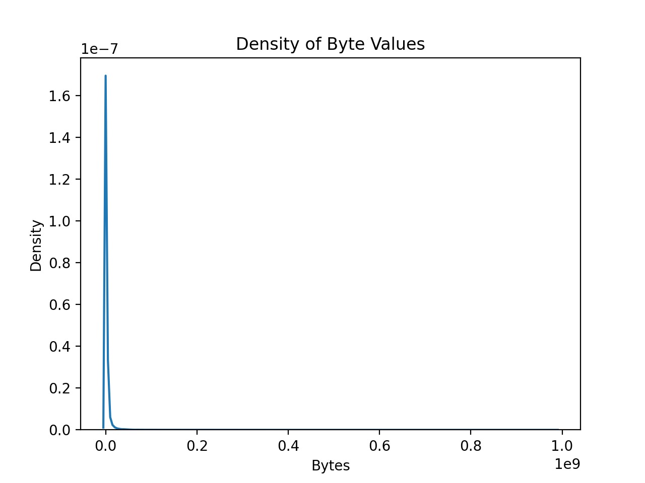
In the context of a distribution, skewness is a measure of how asymmetric the data is. It is clear that the data is extremely skewed to the right, indicated by the density of low byte value observations to the left of the curve, and the massive byte flows shown as one moves along the tail to the right. The outlying values have the effect of increasing the mean of the data. It is important to note that the LSTM models in this project are designed to capture outlying burst flows, although the magnitude of some of the outliers in the SANREN data means that the models may under-predict these observations under testing conditions. The five number summary in the table shows the response values in megabytes and demonstrates the magntitude of outliers in the dataset. The max byte flow is 56 times larger than the average flow.
LSTM Data Preparation
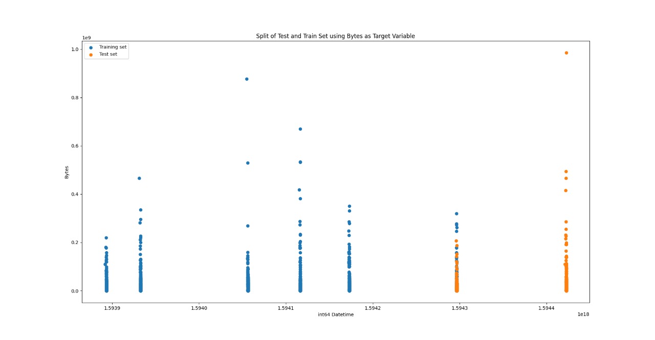
All machine learning algorithms require that the input data is split into training and testing samples. The training data is the sample of the SANREN data that is used to adjust the weights of the LSTM. For our implementation of the LSTMs, the training sample is 64% of the full input sample. Additionally, the training sample is split to produce the validation set. An interesting observation is identified when examining how the validation set is constructed. To ensure the sequential nature of the data, the data is not shuffled when it is split into training and test sets, and it is not shuffled when being split into training and validation sets. The split of data in the sample can be seen on the right. The information provided by the validation set - primarily the out-of-sample MSE of the fitted model - allows the hyperparameters of the model to be adjusted. The model’s evaluation on the validation set becomes more biased as the hyperparameters are adjusted. This is because the model starts to fit the validation set better as the information it provides is incorporated into the model configuration. In our implementation, the validation set is 20% of the training set. Lastly, the test set is the sample of data that is used to provide a truly unbiased evaluation of the final model fit. The test set is used as input to the final, trained model.
Once the train, test and validation sets have been created, LSTM models require that all data is normalised to an equal range of values. The MinMaxScaler from the scikit-learn package scales all variables to a range of 0 to 1. Usually, categorical variables would have to be encoded separately, however, the categorical variables of the SANREN dataset have not been used as predictors in the LSTM models. After the LSTM models have been implemented, the response can be predicted. However, due to the scaled nature of the inputs, the output is also a scaled value between 0 and 1. To convert the LSTM predicted response back to a byte value, a MinMaxScaler is used. The data is then fully prepared, and ready to be given to the LSTM models.
| Min | Q1 | Median | Q3 | Max | Mean |
|---|---|---|---|---|---|
| 0.02 | 0.1 | 0.75 | 2.2 | 177 | 3.15 |
Stacked LSTM
Stacking It Up
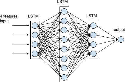
A Stacked LSTM is a Simple LSTM with multiple LSTM layers. Rather than a hidden layer immediately producing a scalar output, the LSTM layer will provide a sequence output to the LSTM layer below it. This implies that the data remains in a three-dimensional format whilst it passes through each of the hidden LSTM layers, before being converted to the required scalar value. Our implementation of a Stacked LSTM in Keras uses three LSTM layers, each with the same number of neurons. Essentially, an LSTM layer returns a sequential output rather than a single scalar. The output layer, the Dense layer in Keras, outputs a scalar prediction based on the three-dimensional input it receives from the LSTM layer above it.
Hyperparameter Tuning
All three of the LSTM models are parameterised functions, meaning that there is an optimal combination of parameters that will minimise the chosen cost function and produce the best performing model [29]. This process is known as hyperparameter tuning. The Simple, Bidirectional and Stacked LSTM models were fitted over a range of hyperparameters. In the context of LSTMs, these parameters are epochs - the number of times the data is passed through the model - and neurons - the number of memory units in each LSTM layer. In this study, each LSTM model was trained using a range of epochs from 25 to 150, with 25 epoch intervals, and with 50 or 100 neurons in each LSTM layer of the model. This resulted in 12 permutations of hyperparameter combinations for each model.
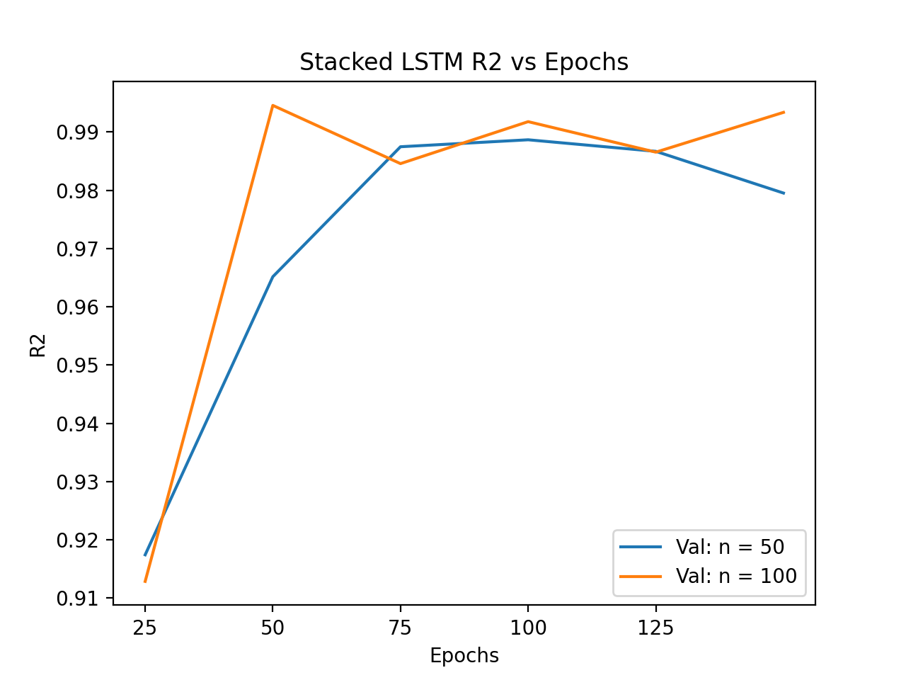
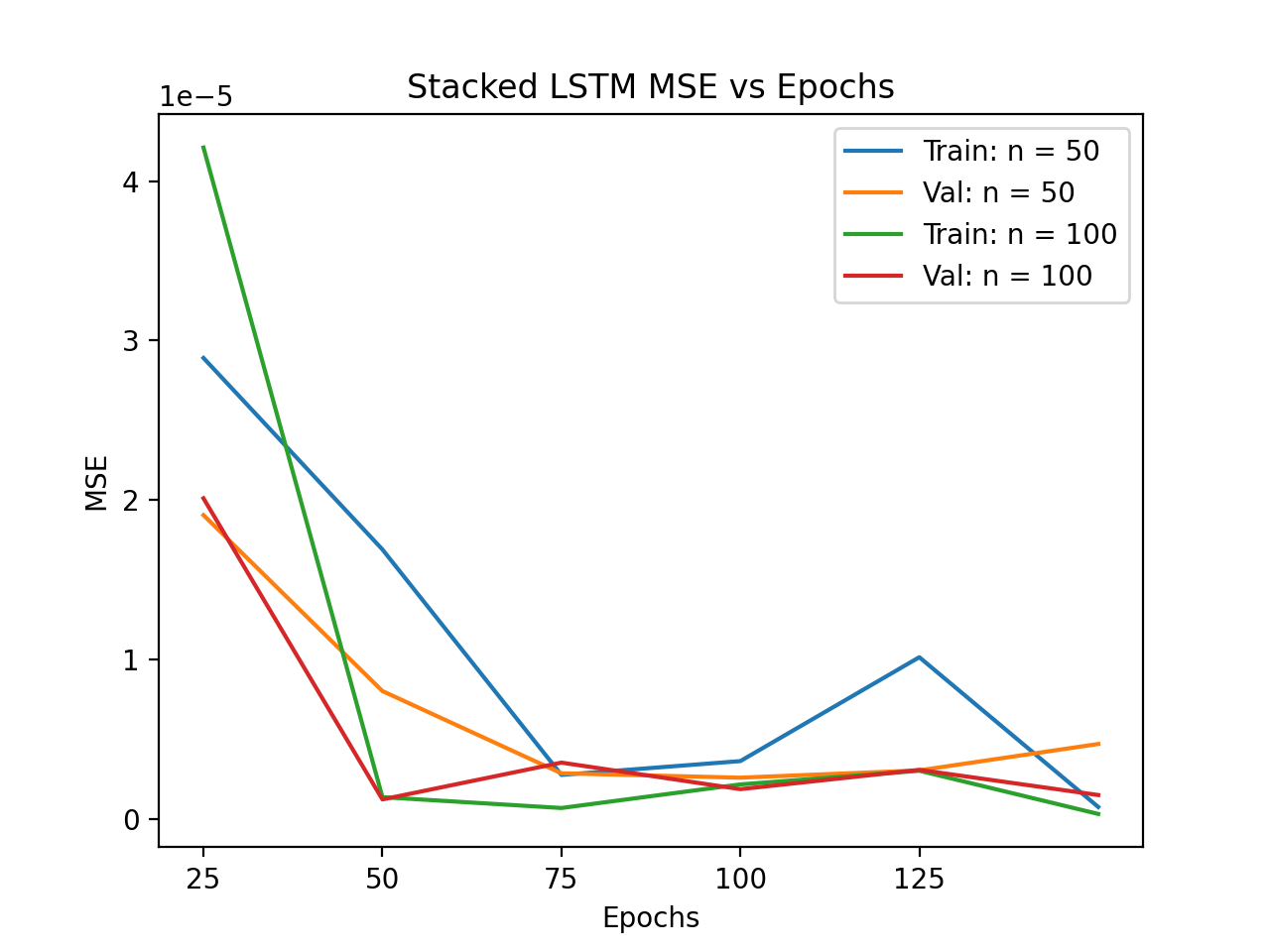
The optimisation of the Stacked LSTM was done using Mean Average Error, Mean Squared Error and Rsquared as assesors of the model's performance on training and validation data. The entire optimisation process can be seen in Antony's Final Paper, although the figures on the left best demonstrates why the Stacked LSTM was optimised the way it was. The validation set MSE at 100 epochs shows that the model is performing well on out of sample data, whereas it starts to overfit if the model is trained over more epochs. The Stacked LSTM model managed to attribute almost all of the variation in the response, Bytes, to the predictors, with an Rsquared value of 99.2% for a 50-neuron model trained over 100 epochs. Therefore, the optimal hyperparameters for the Stacked LSTM model are 100 epochs and 50 neurons. The optimised model was then assessed relative to the optimised Simple and Bidirectional LSTM models. The model comparison and results can be seen on the home page.